ACM Transactions on Graphics, SIGGRAPH 2026

Forget Superresolution, Sample Adaptively (when Path Tracing)

Martin Bálint, Corentin Salaün, Hans-Peter Seidel, Karol Myszkowski

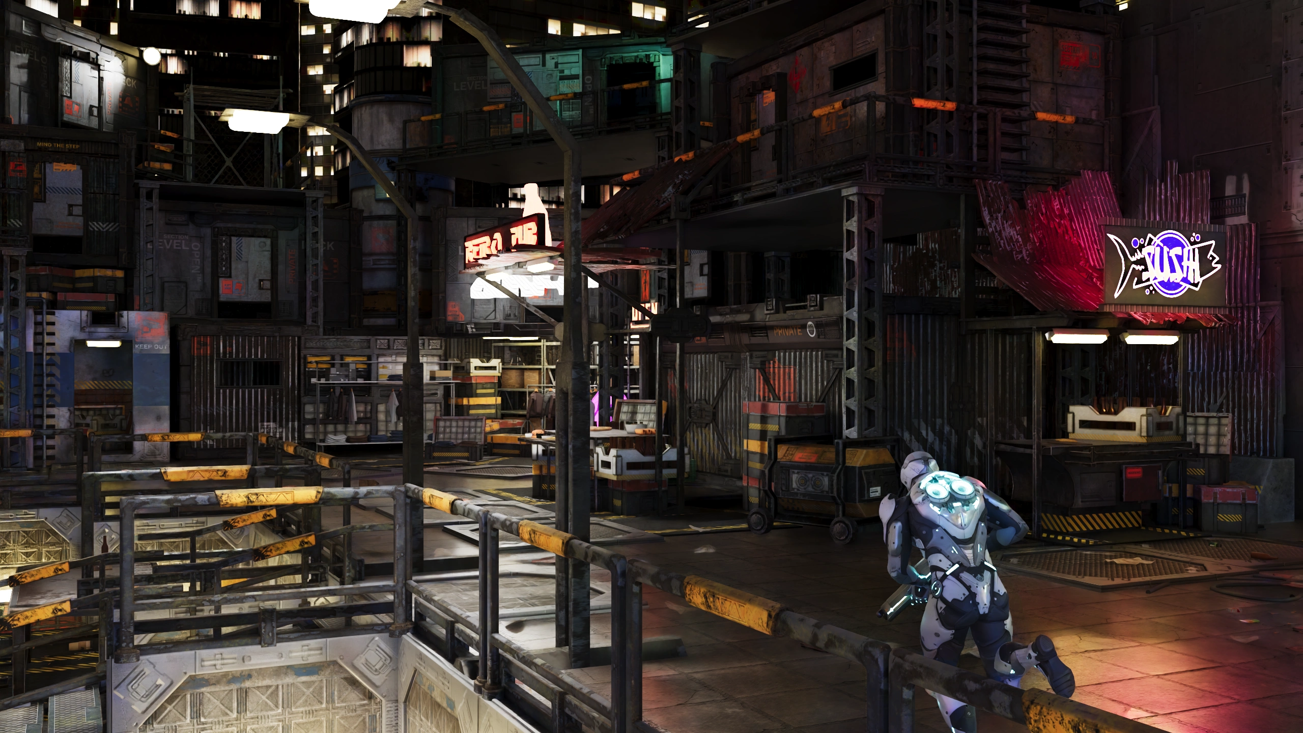
We introduce an end-to-end adaptive sampling and denoising pipeline for sparse real-time path tracing. Our method trains stably despite discrete sampling decisions and uses perceptual, tonemapping-aware optimization to place samples where they matter most. It samples fine structures, specular highlights, and shadows, producing more detailed reconstructions than superresolution or uniform sampling.

Adaptive sparse sampling, trained end to end.
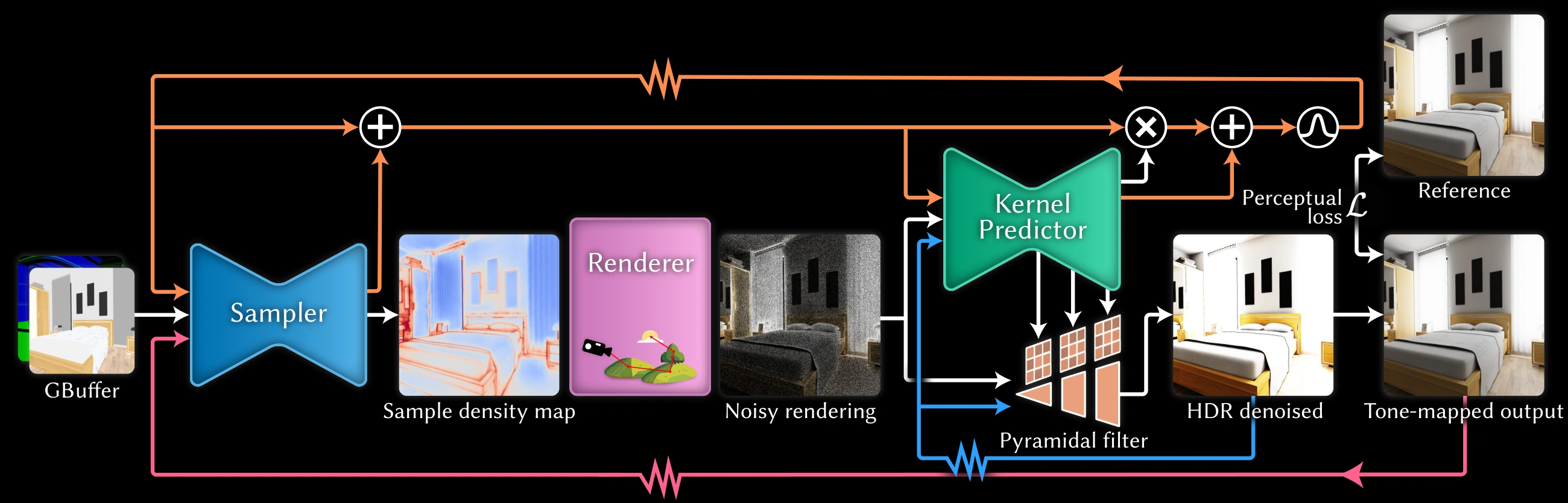
Pipeline overview showing sampler, stochastic discretization, renderer, denoiser, tone mapping, and temporal feedback loops.
Given GBuffer features and temporal data from the previous frame, the sampler network predicts a continuous sample density map. After stochastic discretization, the renderer traces the requested samples, producing a sparse, noisy image. The denoiser network, which shares latent features with the sampler, predicts weights for a pyramidal gather filter. The denoised HDR output is tone-mapped for display and fed back to the sampler in the next frame, closing the perceptual feedback loop.

Previous-frame display feedback guides the sampler.

Shared recurrent features connect sampler and denoiser.

Previous HDR output feeds the denoiser.

Differentiating discrete sampling.

Adaptive sampling chooses which pixels receive path-tracing samples. That choice is discrete, so naive backpropagation gives the sampler little useful signal. We use stochastic rounding with a relaxed estimator, producing gradients that better match finite-difference estimates and remain stable at sparse budgets. This is important for HDR path-traced samples: our clipped ramp has no nonzero tails below the sampling threshold, so rare bright samples cannot shine through pixels that should receive no sample.
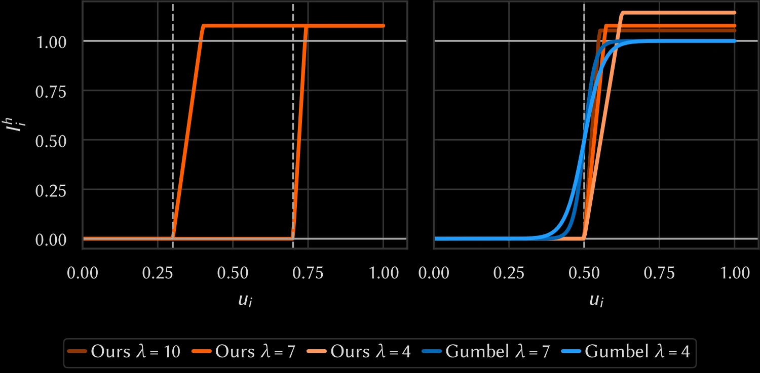
Plot visualizing the relaxed stochastic rounding estimator.
Visualization of our relaxed estimator. On the left, we illustrate the effect of the sampling probability p on the slope of the function at a given temperature parameter λ. On the right, we compare the estimator at a given value of p for different values of λ, along with the Gumbel-Softmax estimator for reference.
Finite difference gradient crop.

Finite difference

Straight-through gradient crop.
Straight-through

Our relaxed estimator gradient crop.

Ours

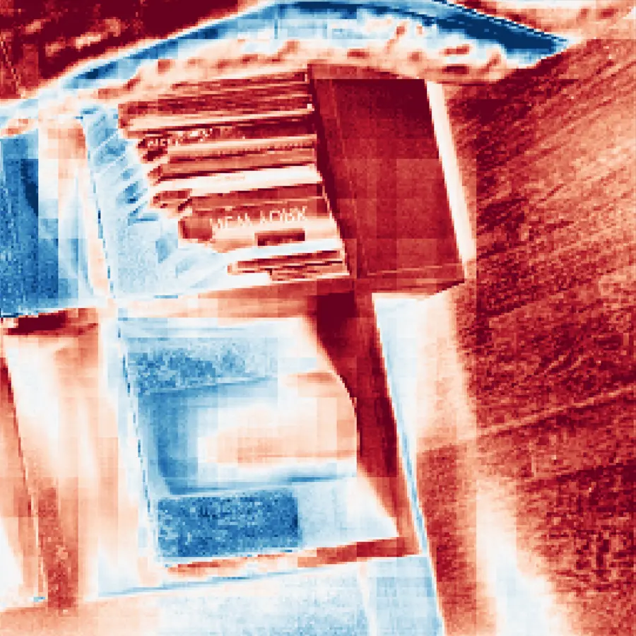
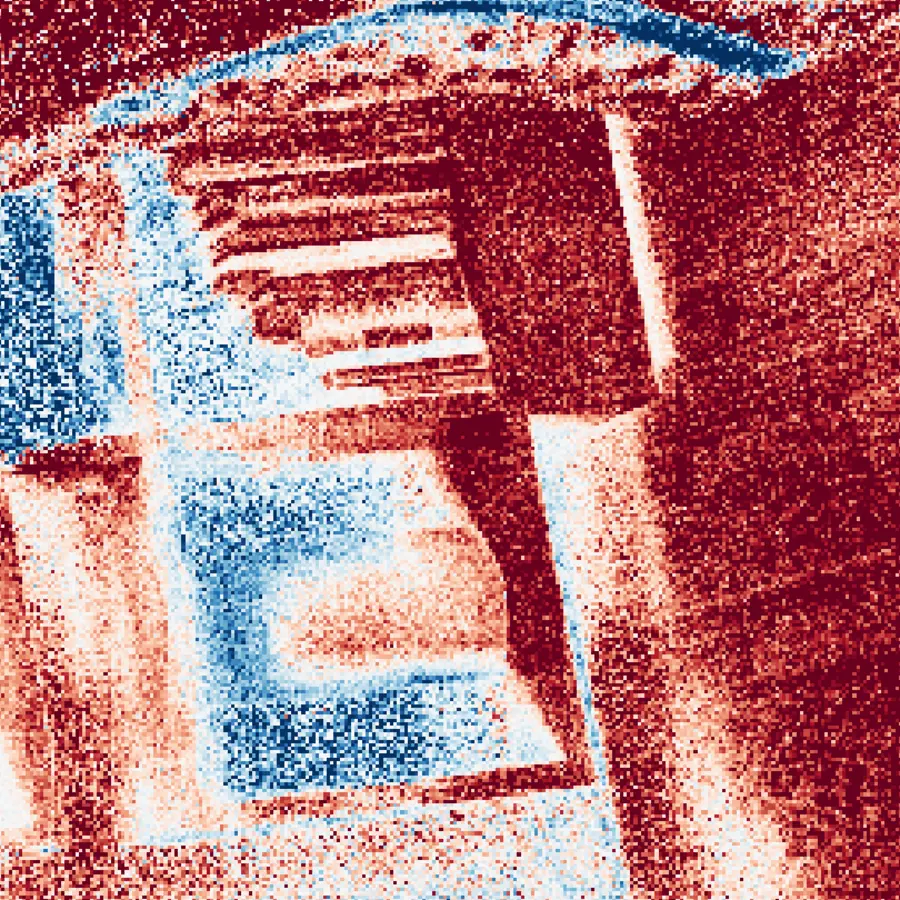
Gradient comparison. We compare the straight-through estimator and our proposed relaxed estimator against the ground-truth gradient estimated via finite differences on a training crop. Our estimator is closest to the finite-difference reference, leading to more stable optimization due to lower gradient bias.

See the paper for tone-mapping-aware training, sparse denoising architecture, ablations, and implementation details.

Sharper details at the same budget.

At the 50 percent superresolution-equivalent budget, adaptive sparse sampling outperforms superresolution and uniform sparse sampling. The visual gains are clearest around fine structures, shadow boundaries, specular highlights, and disocclusions.

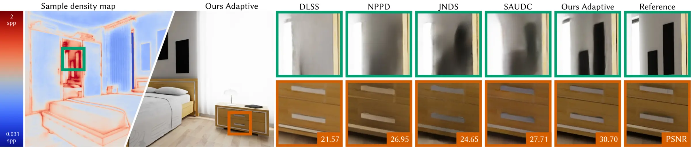
Comparison to baseline methods. 50 percent superresolution equivalent (0.25 spp sparse). We report both SDR/HDR CVVDP versions. Higher is better for all metrics.
Method PSNR MS-SSIM HaarPSI MILO CVVDP SDR/HDR CGVQM
Superresolution with LR inputs
DLSS 22.88 0.8950 0.6195 2.506 6.349 / 6.042 45.01
JNDS 21.92 0.8657 0.5370 2.276 5.621 / 5.508 28.87
Sparse uniform sampling with HR inputs
NPPD 23.92 0.9062 0.6139 2.534 6.393 / 6.407 47.02
Ours Uniform 24.64 0.9183 0.6532 2.640 6.753 / 6.745 55.21
Sparse adaptive sampling with HR inputs
RLSNAS 18.33 0.8077 0.3969 1.986 3.906 / -- -9.08
SAUDC 23.09 0.8848 0.5645 2.250 5.965 / 4.993 38.97
Ours Adaptive 25.41 0.9273 0.6815 2.677 7.056 / 6.972 57.63
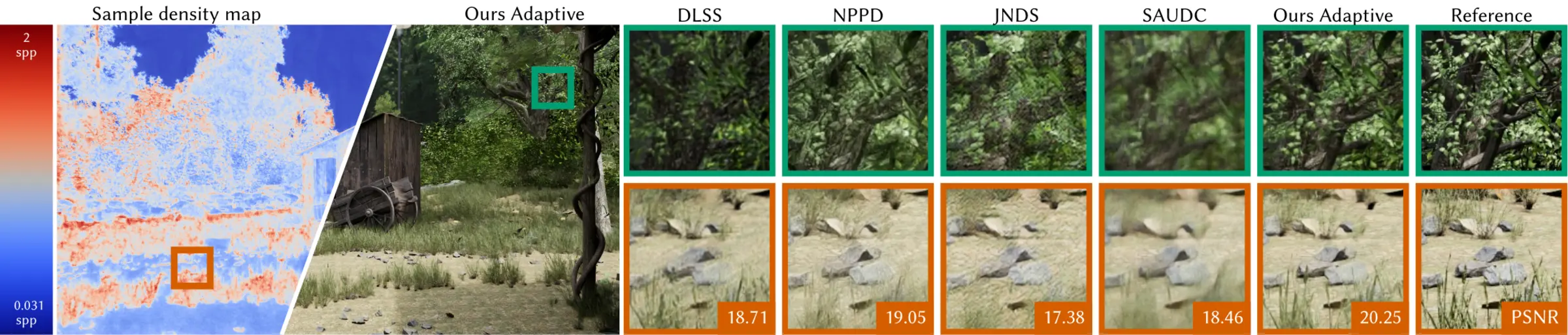
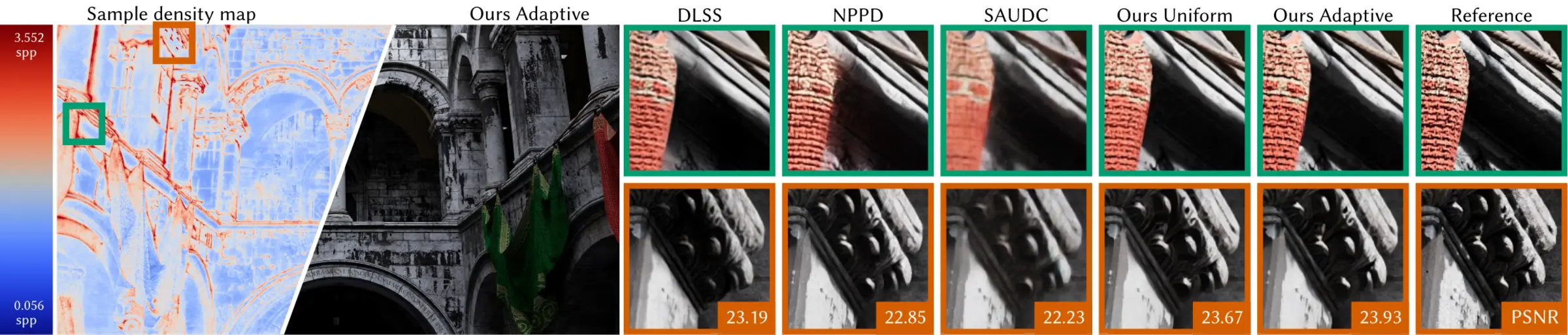
Main bedroom scene comparison at 0.25 samples per pixel. Village scene comparison at 0.25 samples per pixel.
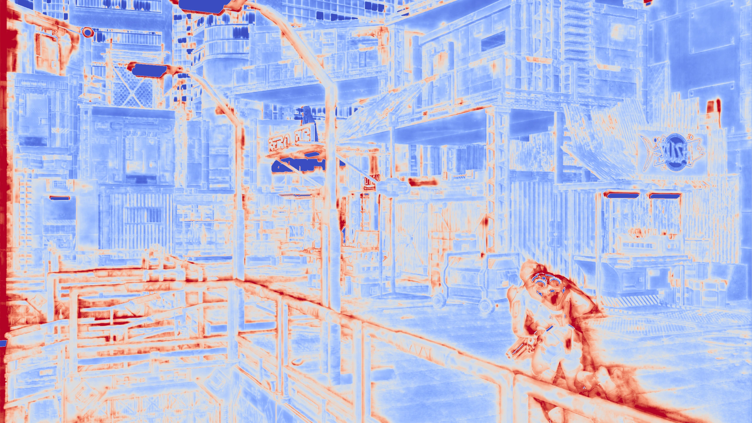
Main comparison at 0.25 spp. We compare our method against baselines at a 50 percent superresolution equivalent budget. Our adaptive method preserves sharp edges and fine texture that superresolution approaches lose due to low-resolution rendering. Other baselines also blur details more than our method. The density maps show our learned sample allocation: blue indicates fewer samples than uniform, red indicates more. PSNR for the full-resolution frame is shown in the bottom-right corner of the orange inset.
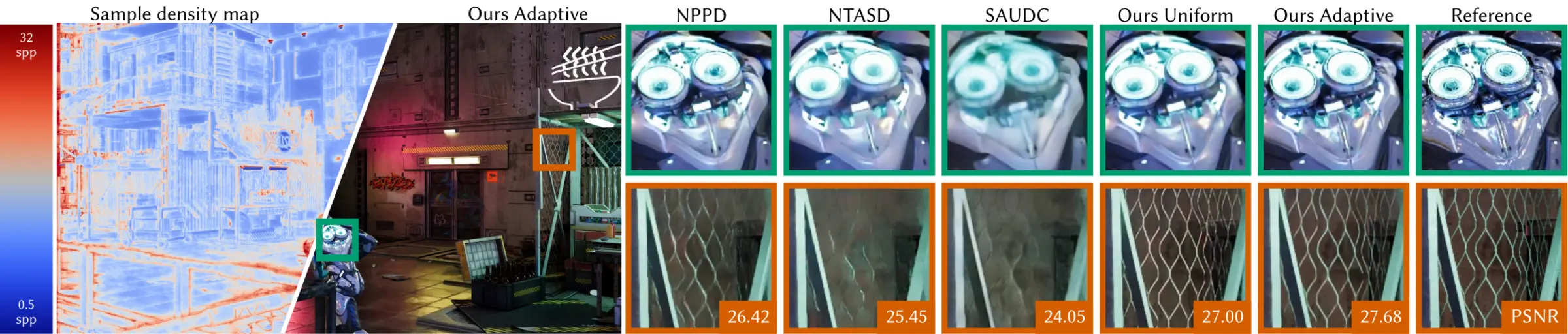
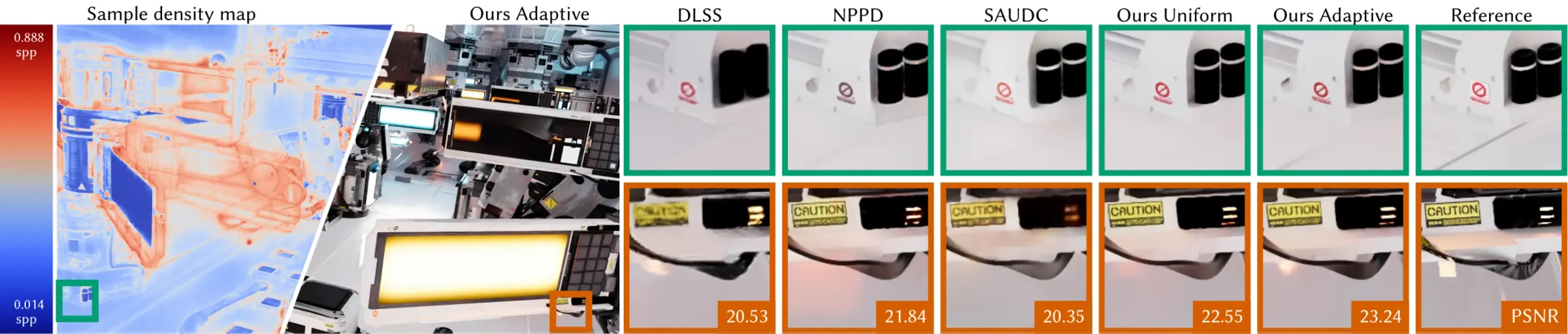
Cyber scene visual comparison at 4.0 samples per pixel. Sponza scene visual comparison at 0.444 samples per pixel. Measure 7 scene visual comparison at 0.111 samples per pixel.
Visual comparison across budgets and scenes. We compare our method against baselines at 4.0 spp (top), 0.444 spp (middle), and 0.111 spp (bottom). Our adaptive method recovers fine details that competitors blur. The sample density maps show our learned sample allocation: blue indicates fewer samples than uniform, red indicates more. PSNR for the full-resolution frame is shown in the bottom-right corner of the orange inset. Our sampler concentrates samples on perceptually important regions such as edges and specular reflections while reducing allocation in smooth areas.

Robust adaptive sampling. (Finally.)

Adaptive sampling has a reliability problem: with a fixed total budget, allocating more samples to one region means taking them from another. We compare the best- and worst-performing regions against uniform sampling. The sampler gives up samples mostly in smooth, low-contrast areas where errors are hard to see, while spending them on fine geometry and high-error regions where the gain is visible.
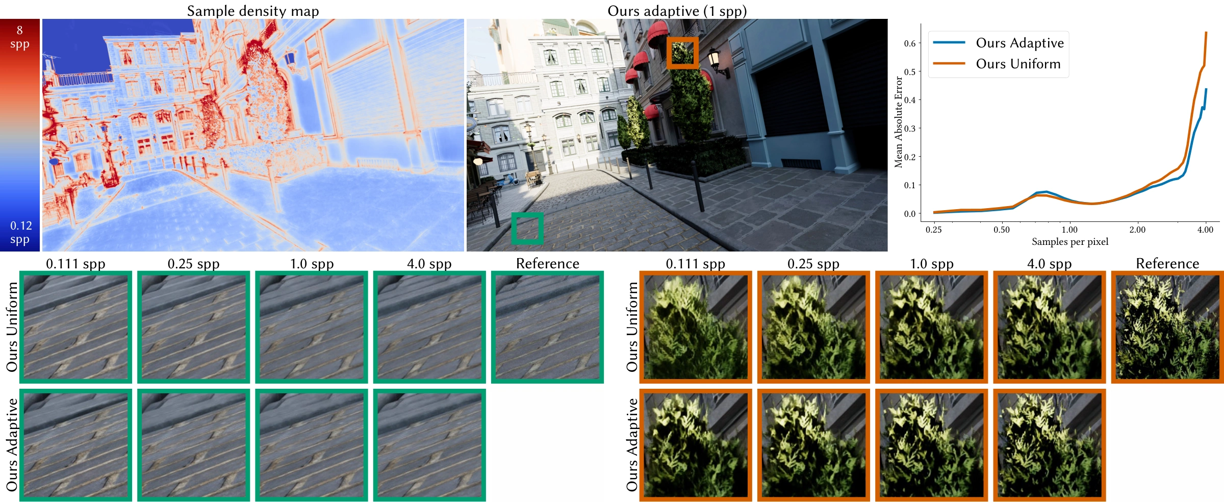
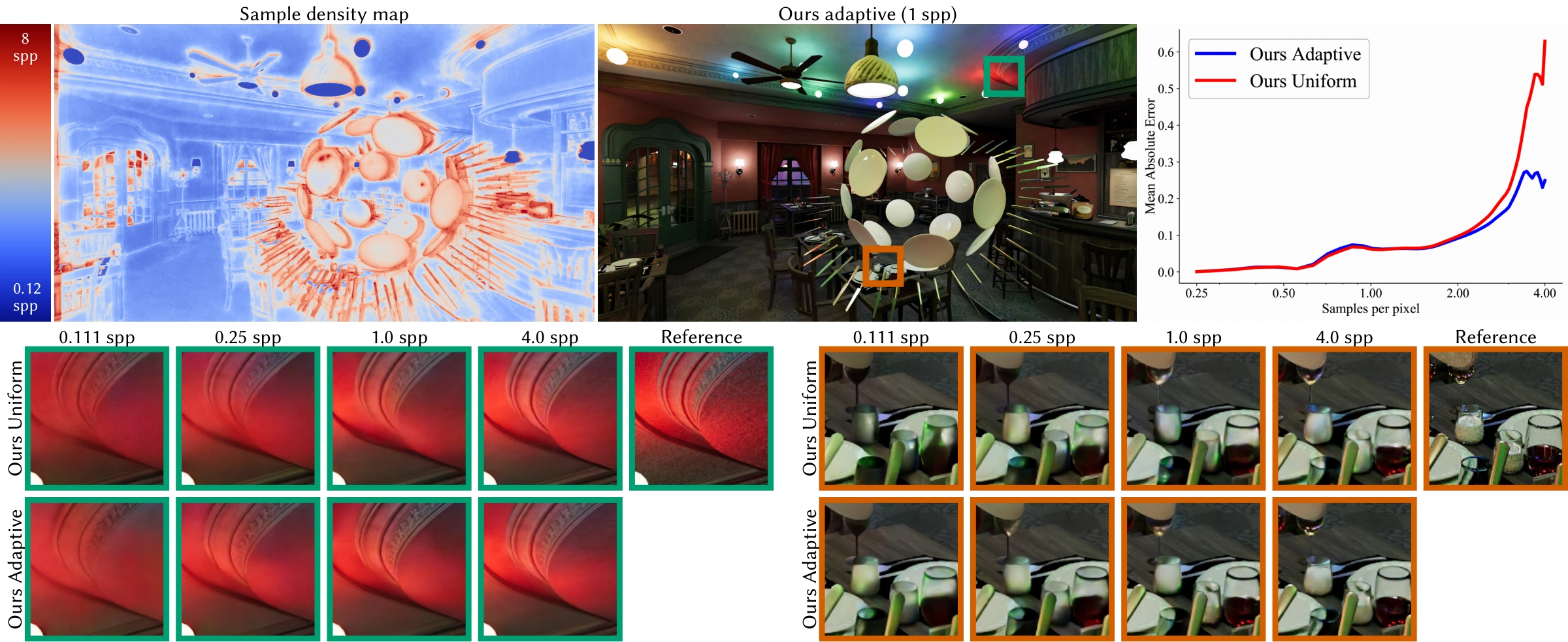
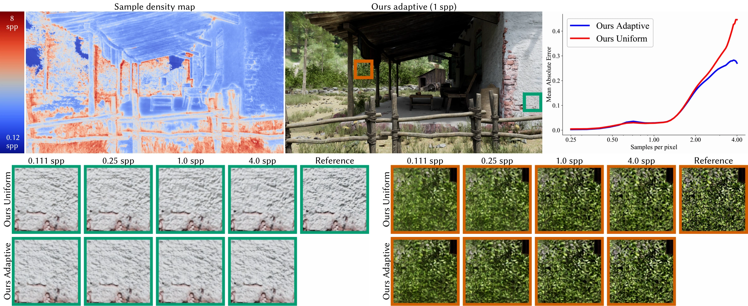
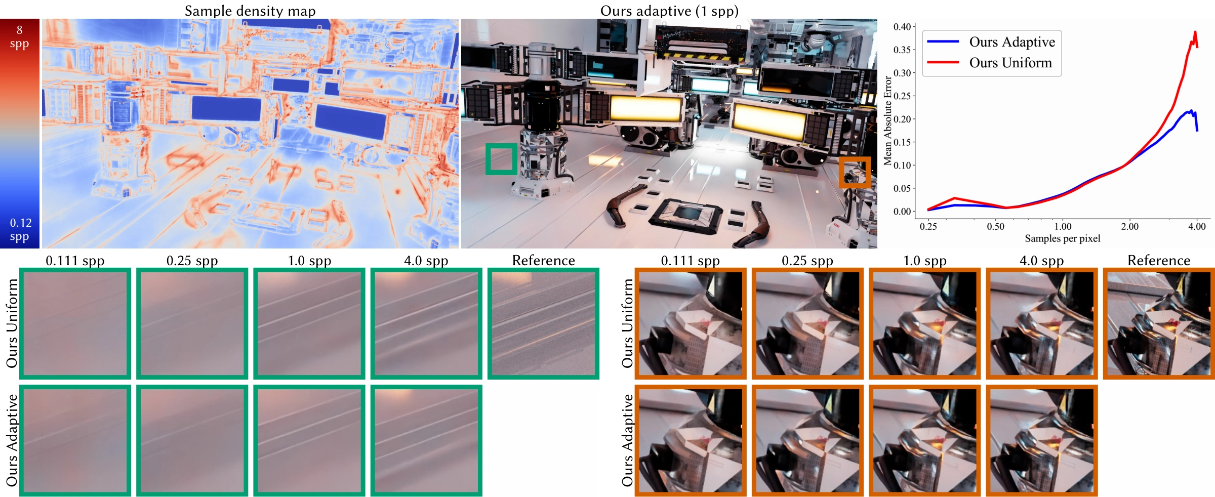
Best- and worst-case robustness analysis comparing adaptive and uniform sampling.
Best- and worst-case robustness analysis. This figure compares, for the same scene, the best- and worst-performing regions of our adaptive sampling method relative to uniform sampling. The green inset highlights the crop where uniform sampling performs best, while the orange inset highlights the crop where adaptive sampling performs best. The comparison shows that adaptive sampling better reconstructs fine details, while only slightly underperforming in more uniform regions. The plot on the right illustrates the mean absolute error as a function of relative sampling rate. When adaptive sampling allocates fewer samples than uniform sampling (left side of the plot, sampling ratio < 1), the error increases only marginally. In contrast, when adaptive sampling allocates more samples than uniform sampling (right side, sampling ratio > 1), the error reduction is substantial. This demonstrates that the sampler successfully focuses computation on high-error regions, leading to an overall improvement in image quality.

BibTeX

@article{balint2026fssa,
  title = {Forget Superresolution, Sample Adaptively (when Path Tracing)},
  author = {Balint, Martin and Salaun, Corentin and Seidel, Hans-Peter and Myszkowski, Karol},
  journal = {ACM Transactions on Graphics},
  year = {2026},
  volume = {45},
  number = {4},
  article = {90},
  doi = {10.1145/3811377}
}